The NIH's "Rule of 21" — Part 2
The doctrine of economy, in general, treats of the relations between utility and cost. That branch of it which relates to research considers the relations between the utility and the cost of diminishing the probable error of our knowledge. Its main problem is, how, with a given expenditure of money, time, and energy, to obtain the most valuable addition to our knowledge.
Charles Sanders Peirce (1879)
Note on the Theory of the Economy of Research
tl;dr summary: The NIH had planned to limit the number of their grants that any one scientist may hold concurrently in order to optimize scientific return on investment. To determine optimal funding allocation, they have estimated a "production function" for NIH investigators that maps funding input to research output. But this production function has been inferred inappropriately. Rather than comparing how individual investigators respond to changes in funding, they compare outputs across different investigators receiving differing amounts of funding. The problem with this approach is that if review panels are doing anything useful, investigators' funding will vary systematically with their abilities to convert funding into impactful work. As a result, the production function that the NIH has inferred from data and which they use in their optimization calculations is unlikely to adequately predict the consequences of actual funding changes.
Introduction
In Part 1 of this case study we looked at the way in which data visualization on a log-log scale contributed to incorrect inferences about decreasing returns. In this second part of the case study, we will consider the underlying logic around optimizing the returns on investment for NIH grant funds.
Recall the basic story. In an effort to reform NIH funding regulations, Mike Lauer and colleagues:
- Used data on funding and research impact of individual investigators to estimate a production function relating funding input (measured at RCI) to research output (measured as RCR).
- Used this production function to make arguments about funding based on optimality considerations. In particular, they fit a curve through their data, and noted decreasing marginal returns of research investment on research impact.
- Proposed the so-called "Rule of 21" which caps the number of grants a single investigator can hold concurrently.
Unfortunately, in doing so they made a mess of interpreting their log-log plots (Part 1), and they seem overly concerned with marginal return rather than average return . But these issues are correctable.
There is a more fundamental problem with the approach: the production function does not predict the effect of increased funding on any individual investigator. Why? The problem is that Lauer estimated the production function using inputs and outputs from investigators who differ systematically with respect to their production abilities. Or to put it another way, the investigators from whom the production function has been estimated have already been selected to receive funding based upon their productivity.
A baseball analogy
Often an analogy can make complex ideas obvious. Readers who know even a wee bit about baseball may find the following example useful. The rest of you can safely skip ahead.
—
Imagine for a moment that you are the manager of a struggling Major League Baseball club, sitting in your weekly meeting with the team owner. Twitching with excitement, he pulls out the graph below, compiled from the complete pitching record for all 30 MLB teams.
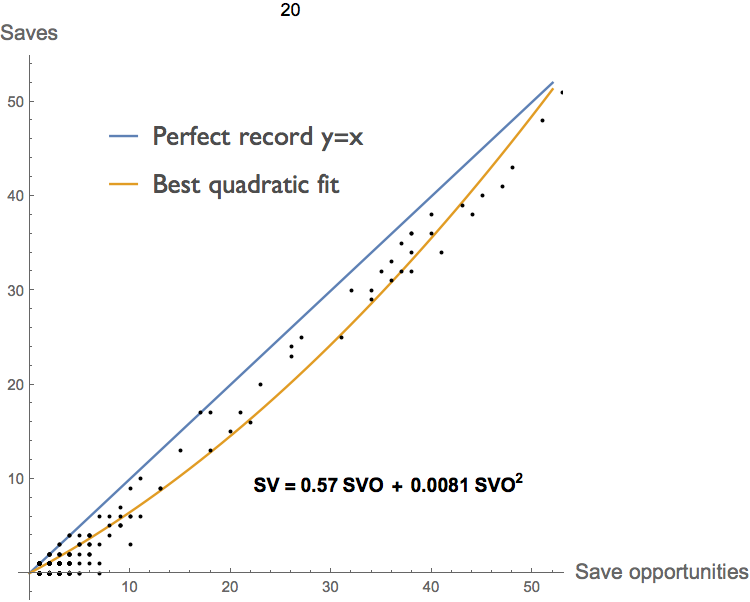
"Look at this," he exclaims, I had one of our stats guys pull together a graph of saves against save attempts. The more save attempts a guy is given, the more saves he gets, of course. But he also gets a higher percentage of saves. There are increasing returns to scale from pitching more innings!"
"Your problem," he continues, "is that you're not pitching the bullpen guys enough! But don't worry — I had the general manager trade a couple of your relievers for a reserve infielder and a third round draft pick. This way you can give the remaining guys more time on the mound."
"You idiot!", you roar, not pausing to realize that it's your boss that your are shouting at, "I've already got our pitchers throwing as many innings as they can. You're not going to turn Joe Journeyman into Mariano Rivera by doubling his innings. You're just going to blow a lot of saves and ruin his arm in the process."
—
In this story the owner's mistake is pretty easy to see. The pitchers are neither identical nor assigned a number of innings at random. If the manager is even remotely competent, the better pitchers will get more innings, and weaker pitchers will get fewer. Guys with iron arms may throw every day; a veteran reliever recovering from arm trouble might throw only once a week. In other words, the pitchers that make up the curve have already been selected on endurance and pitching ability.
As a result, the composite curve in the figure above, assembled from the records of many different individuals, is next to useless as a predictor of how any individual pitcher will respond to changes in the number of innings he is asked to pitch. If pitchers had been assigned a number of innings at random, a composite curve like this could be useful for prediction . But instead, the manager has already attempted to optimize each pitcher's production in a manner specific to that individual. For example, each individual pitcher might have a production curve more like that sketched in red below.
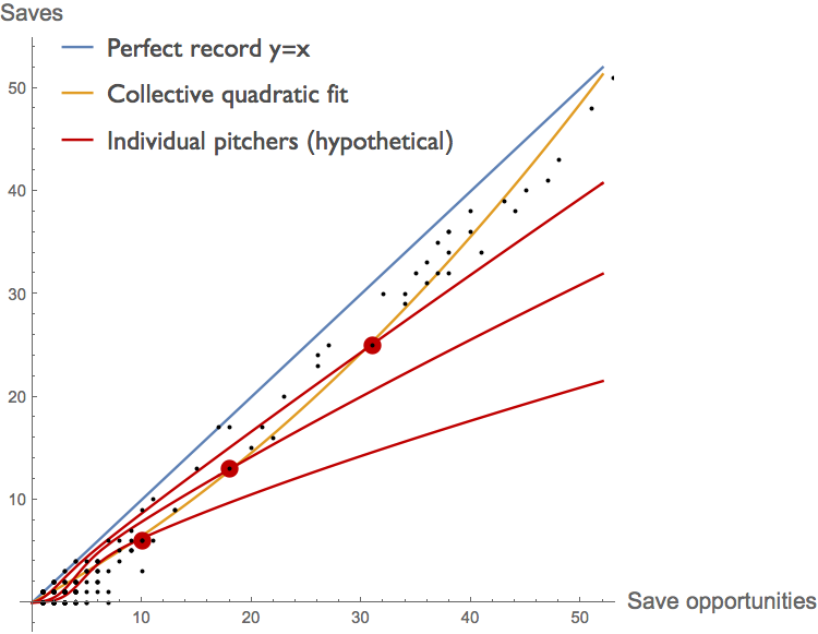
In this scenario, the job of the manager is to get as close to the blue \(x=y\) line as he can, using his best relievers as much as possible without over-pitching them. We don't expect him to do this perfectly, but nor do we expect him to issue pitching assignments at random. As a result, the trajectory of the best fit to the composite data (yellow) does not reflect the response of individual pitchers to chances in their pitching loads. They need not even have the same concavity. Here the yellow composite curve is convex, whereas the hypothetical curves for individual pitchers, in red, are all concave once we get beyond a half-dozen save opportunities or so.
In the following section, we will see that the NIH is making an analogous mistake when they use a composite graph to predict the effects of changes in the funding that they provide to individual investigators.
Back to biomedical research
Unlike the idealized firms in an economics textbook, different principal investigators will differ in their capacities to convert funding into research impact. A simple way of conceptualizing this might be to imagine that each researcher has an unobserved scalar "research ability" that determines how efficiently she converts funding (RCI) into research impact (RCR). Researchers with higher research abilities would have steeper production functions.
The production function that the NIH has inferred is not the production function of any single individual, but rather is derived from a composite of investigators of differing abilities. As in our baseball example, this would not necessarily be a problem if funding levels and ability levels were uncorrelated. But unless grant review panels are no better that a lottery, their efforts ensure that investigators of higher ability receive more funding on average. Thus in the data that the NIH has used, lower-ability investigators tend to receive smaller amounts of funding and higher-ability investigators tend to receive larger amounts of funding.
Another way to view this is to note that, like a baseball manager assigning different pitching loads to different pitchers, the panel review process has already taken an initial — if very rough – crack at allocating funding across individual investigator to maximize total research output.
The key consequence of this is that on average, tripling the funding to a focal investigator with one R01 should increase that investigator's output, but it should not increase all the way to the average output of the other investigators who already hold 3 R01s. This is because NIH's can increase the funding of a 1-R01 investigator to the level of a 3-R01 investigator, but its funding decisions do not increase a 1-R01 investigator's ability to the average ability of 3-R01 investigators.
What does this mean for the Rule of 21? It means that shifting resources away from highly funded investigators and redirecting them to less well-funded investigators is unlikely to provide the benefits the NIH expects given their inferred production function. (For a formal explanation of why this happens, see the endnote). Giving an R01 to an investigator who was previously unfunded does not give an expected return as high as the average return from 1-R0 investigators, because on in expectation this previously unfunded investigator has a lower ability than the current 1-R01 investigators. Similarly, giving a second R01 to 1-R01 investigator does not yield the expected return of a 2-R01 investigator, because in expectation the 1-R01 investigator does not have as high of an ability as the 2-R01 investigators.
The figure below illustrates an example of how this might work. In this figure, the individual production functions (red, orange, and yellow curves) all exhibit constant returns, but the collection of all investigators at their current funding levels (yellow, orange, and red dots) generates a blue sigmoid function similar to that which the NIH inferred from their data.
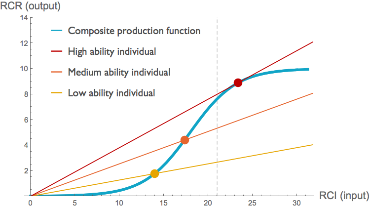
Applying something the Rule of 21 here (dashed grey line), we would take funding from the high-ability investigator (red dot) and give instead to a low- or medium-ability individual. Looking at marginal returns along the blue composite production function, it seems as if doing so would increase output. The slope of the blue curve is approximately 1.1 and 2.4 times larger at the yellow and orange points respectively than it is at the red point. But looking at the individual productions functions, we see that taking resources from the high-ability investigator would substantially decrease output. The slope of the high-ability investigator's production function at the current funding level is four times that of the low ability individual, and over 60% higher than that of the medium ability individual.
In this particular example with linear production functions, transferring funds from well-funded investigators to less well-funded investigators always decreases total productivity. That will not be true in general; it depends on the slopes of the individual production functions at the funding levels investigators are currently receiving.
But the point is that given the likely correlation between the funding that individuals currently receive and the shape of their individual production functions, we have little cause to believe that the composition production function reflects the shape of the individual functions. Changes to funding levels will shift along individual production functions and thus efforts to optimize output based on the composite function are fundamentally misguided. This is the core mistake that undermines the logic behind the NIH's Rule of 21.
Conclusion
In Part 1 of this case study we saw that the NIH made unsubstantiated claims in an effort to justify their Rule of 21, based on confusion between concavity on a log-log plot and concavity on a linear plot. Here in Part 2, we have seen that the approach of estimating a composite production function, and then trying to optimize output given this function, has a fatal flaw. The problem is that, if review panels work at all, we expect more highly funded investigators to have steeper production functions. As a result, a transfer of resources from highly funded investigators to less well-funded investigators is likely to generate less of an increase in total output than the composite production function suggests. Doing so may even decrease total output.
The NIH didn't need to make these fallacious arguments to support the Rule of 21. If the NIH had simply declared that their objective is not to maximize the short-term citation impact of their funding, but instead to diversify their research portfolio in the interest of exploring a broader range of approaches and directions, this would be a reasonable argument. Their mistake, in our opinion, was to attempt a justification on optimality grounds in the first place. By framing RCR maximization as a reasonable goal, they have painted themselves into a corner with regard to alternative objectives. Once people realize that the Rule of 21 doesn't optimize output in the way that the Lauer and colleagues have claimed, the NIH is left with little option but to admit either that they made a horrible mess of the optimization, or that optimizing citation impact in the form of RCR was never the aim in the first place.
Carl T. Bergstrom
University of Washington
June 23, 2017
Note regarding author's response: As with all scholarly authors whose work appears in one of our case studies, Mike Lauer was offered the opportunity to publish a response here at the end of our article. We have not received a reply.
Endnote
Consider a model in which each investigator has an ability level \(a \in \mathcal{A} \) and receives funding \(x \in \mathcal{X}\) from the NIH. The return on the NIH's investment in a given investigator is given by some function \(f(x,a)\) which we presume to be non-decreasing in both arguments. The actual allocation of funding to investigators is described by a joint density function \(\pi(x,a)\). Because \(a\) is unobservable (or at least unobserved), NIH does not know \(f(x,a)\) or \(\pi(x,a)\), nor do they know the marginal distribution of abilities \(\pi(a)\). They do know the marginal distribution \(\pi(x)\) and the average return across all ability levels \(a\) from each funding level \(x\): \(E_A[f(x,a)|x]\).
If the NIH wants to understand the consequences of changing the distribution of funding amounts, they would ideally like to calculate something like the marginal return with respect to \(x\), averaged over all abilities: \[g(x)=\int_{a\in\mathcal{A}}\frac{\delta}{\delta x} f(x_i,a_i)\, \pi(a)\, da,\] But as noted above, they don't have the information they need to compute this. The approach that the NIH has taken is to approximate \(g(x)\) with a function that can be computed from observed data: $$\begin{eqnarray} h(x)&=& \frac{d}{dx} E_A[f(x,a)|x] \nonumber \\ &=& \frac{d}{dx}\int_{a\in\mathcal{A}} f(x,a)\, \pi(a|x) \,da \nonumber \\ &=& \int_{a\in\mathcal{A}} \frac{\delta}{\delta x} \left[ f(x,a)\,\pi(a|x)\right]\,da \nonumber \end{eqnarray}$$ If \(a\) and \(x\) are independent, then \(h(x)=g(x)\). This follows from the fact that under independence, \(\pi(a|x)=\pi(a)\) and thus $$\begin{eqnarray} h(x)&=& \int_{a\in\mathcal{A}} \frac{\delta}{\delta x} \left[ f(x,a)\,\pi(a)\right]\,da \nonumber \\ &=& \int_{a\in\mathcal{A}} \frac{\delta}{\delta x} f(x,a) \cdot \pi(a)\,da \nonumber \\ &=& g(x). \nonumber \end{eqnarray}$$ If however \(a\) and \(x\) are correlated, as we would expect if the review panels are doing anything constructive, \(f(x,a)\,\pi(a|x) \neq f(x,a)\,\pi(a)\). Thus the function \(h(x)\) that the NIH infers from data may not be a good estimate of the marginal return on changes from funding \(g(x)\) they would like to know for planning purposes.